Basic Office Technologies

Beginners level

Unit 1: Give solutions to your clients: Use an Excel sheet

AIMS & OBJECTIVES

  1. The purpose of this unit is to enhance migrants’ ICT skills, by offering them the opportunity to explore the use of Excel Sheet. Learners will be able to gain basic knowledge on understanding and applying data.  
  2. The presentation covers basics of Excel use and  enables understanding on variety of possibilities Excel contains to be good to use while giving solutions to the clients.

LEARNING OUTCOMES

LOut1: know the basic features and possibilities of Excel 

LOut2: understand and navigate Excel worksheet

LOut3: apply and use Formulas and Variety of Functions for various solutions 

LOut4: demonstrate skills to choose, combine and apply the variety of Excel templates

LOut5: present data in charts

LOut6: create presentation of solutions and share it with the clients

KEYWORDS

  • Excel,
  • Cells,
  • Workbook,
  • Ribon,
  • Toolbar,
  • Worksheet,
  • Formulas,
  • Functions,
  • Data,
  • Charts,
  • Templates

1.1 Introduction

Excel is a tool that allows you to enter quantitative data into an electronic spreadsheet to apply one or many mathematical computations. These computations ultimately convert that quantitative data into information.


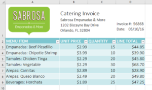
Excel is a spreadsheet program that allows you to storeorganize, and analyze information. While you may believe Excel is only used by certain people to process complicated data, anyone can learn how to take advantage of the program’s powerful features. Whether you’re keeping a budget, organizing a training log, or creating an invoice, Excel makes it easy to work with different types of data.

1.2 Working with the Excel environment

  1. Locate Excel on your computer.
  2.  Click Microsoft Excel to launch the Excel application.

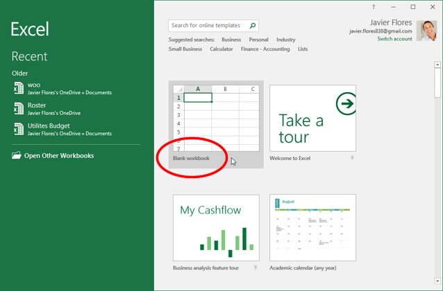
When you open Excel for the first time, the Excel Start Screen will appear. From here, you’ll be able to create a new workbook, choose a template, and access your recently edited workbooks.

From the Excel Start Screen, locate and select Blank workbook to access the Excel interface.

Blank Workbook

Your workbook should already be maximized (or shown at full size) once Excel is started. If necessary locate the Maximize button as shown.

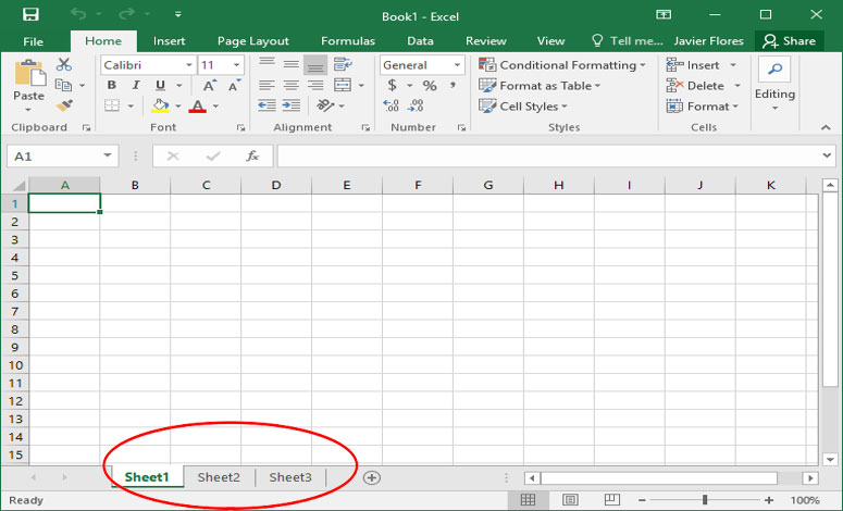
The Excel Workbook is an Excel file that contains one or more worksheets (sometimes referred to as spreadsheets). Excel will assign a file name to the workbook, such as Sheet1Sheet2Sheet3, (or Book1, Book2..)and so on, depending on how many new workbooks are opened.

The Ribbon

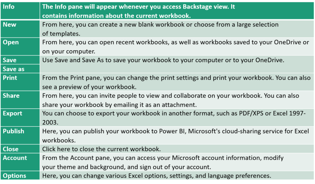
The Ribbon and Quick Access Toolbar are where you will find the commands to perform common tasks in Excel. The Backstage view gives you various options for saving, opening a file, printing, and sharing your document.

Excel Ribbon contains multiple tabs, each with several groups of commands. You will use these tabs to perform the most common tasks in Excel.

Minimizing or Maximizing the Ribbon – Hold down the CTRL key and press the F1 key.

Command Overview for Each Tab of the Ribbon

File: Also known as the Backstage view of the Excel workbook. Contains all commands for opening, closing, saving, and creating new Excel workbooks. Includes print commands, document properties, e-mailing options, and help features. The default settings and options are also found in this tab.

Home: Contains the most frequently used Excel commands. Formatting commands are found in this tab along with commands for cutting, copying, pasting, and for inserting and deleting rows and columns.

Insert: Used to insert objects such as charts, pictures, shapes, PivotTables, Internet links, symbols, or text boxes.

Page Layout: Contains commands used to prepare a worksheet for printing. Also includes commands used to show and print the gridlines on a worksheet.

Formulas: Includes commands for adding mathematical functions to a worksheet. Also contains tools for auditing mathematical formulas.

Data: Used when working with external data sources such as Microsoft® Access®, text files, or the Internet. Also contains sorting commands and access to scenario tools.

Review: Includes Spelling and Track Changes features. Also contains protection features to password protect worksheets or workbooks.

View: Used to adjust the visual appearance of a workbook. Common commands include the Zoom and Page Layout view.

* Each tab will have one or more groups.

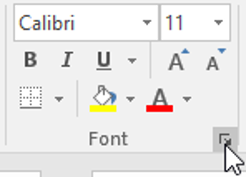
* Some groups will have an arrow you can click for more options.

Click a tab to see more commands.

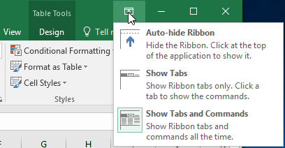
You can adjust how the Ribbon is displayed with the Ribbon Display Options.

The Quick Access Toolbar

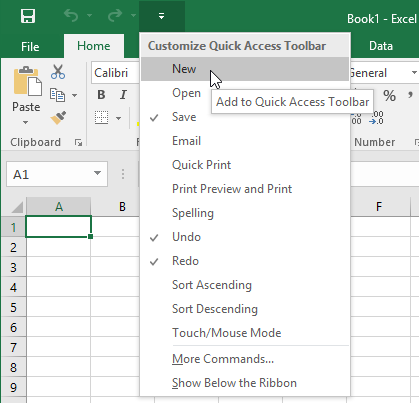
Located just above the Ribbon, the Quick Access Toolbar lets you access common commands no matter which tab is selected. By default, it includes the SaveUndo, and Repeat commands. You can add other commands depending on your preference.

To add commands to the Quick Access Toolbar:

  1. Click the drop-down arrow to the right of the Quick Access Toolbar.
  2. Select the command you want to add from the drop-down menu. To choose from more commands, select More Commands.
  3. The command will be added to the Quick Access Toolbar.

How to use Tell me:

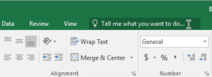
The Tell me box works like a search bar to help you quickly find tools or commands you want to use.

  1. Type in your own words what you want to do.
  2. The results will give you a few relevant options. To use one, click it like you would a command on the Ribbon.

Worksheet views

Excel 2016 has a variety of viewing options that change how your workbook is displayed. These views can be useful for various tasks, especially if you’re planning to print the spreadsheet. 

To change worksheet views, locate the commands in the bottom-right corner of the Excel window and select Normal view, Page Layout view, or Page Break view.

A – Normal view is the default view for all worksheets in Excel.

B – Page Layout view displays how your worksheets will appear when printed. You can also add headers and footers in this view.

C – Page Break view allows you to change the location of page breaks, which is especially helpful when printing a lot of data from Excel.

1.3 Working with Cells and Sheets

Whenever you work with Excel, you’ll enter information—or content—into cells. Cells are the basic building blocks of a worksheet. You’ll need to learn the basics of cells and cell content to calculate, analyze, and organize data in Excel.

Understanding cells

Whenever you work with Excel, you’ll enter information—or content—into cells. Cells are the basic building blocks of a worksheet. You’ll need to learn the basics of cells and cell content to calculate, analyze, and organize data in ExcelEvery worksheet is made up of thousands of rectangles, which are called cells. A cell is the intersection of a row and a column—in other words, where a row and column meet.

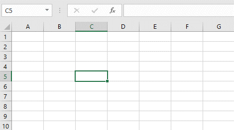
Columns are identified by letters (A, B, C), while rows are identified by numbers (1, 2, 3). Each cell has its own name—or cell address—based on its column and row. In the example below, the selected cell intersects column C and row 5, so the cell address is C5.

To select a cell range:

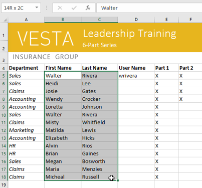
Sometimes you may want to select a larger group of cells, or a cell range.

1. Click and drag the mouse until all of the adjoining cells you want to select are highlighted. In our example, we’ll select the cell range B5:C18.

2. Release the mouse to select the desired cell range. The cells will remain selected until you click another cell in the worksheet.

Cell content

Any information you enter into a spreadsheet will be stored in a cell. Each cell can contain different types of content, including textformattingformulas, and functions.

Text: Cells can contain text, such as letters, numbers, and dates.

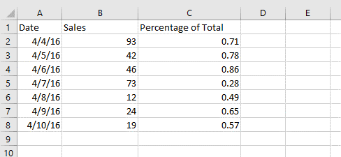
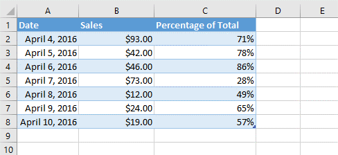
Formatting attributes: Cells can contain formatting attributes that change the way letters, numbers, and dates are displayed. For example, percentages can appear as 0.15 or 15%. You can even change a cell’s text or background color.

What are number formats?

Number formats tell your spreadsheet exactly what type of data you’re using, like percentages (%), currency ($), times, dates, and so on.  For example, the date format tells the spreadsheet that you’re entering specific calendar dates. This allows the spreadsheet to better understand your data, which can help ensure that your data remains consistent and that your formulas are calculated correctly.

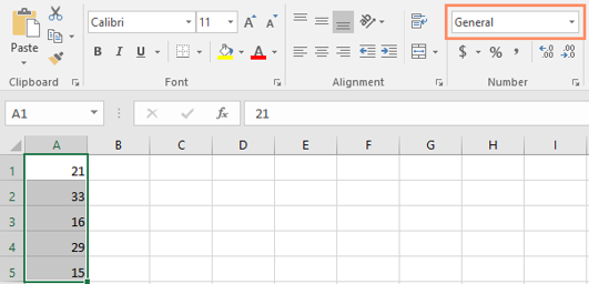
You’ll apply number formats by selecting cells and choosing the desired formatting option. There are two main ways to choose a number format:

1. Go to the Home tab, click the Number Format drop-down menu in the Number group, and select the desired format.

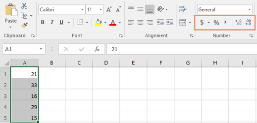
2. You can also click one of the quick number-formatting commands below the drop-down menu.

You can also select the desired cells and press Ctrl+1 on your keyboard to access more number-formatting options.

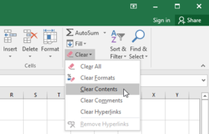
To delete (or clear) cell content:

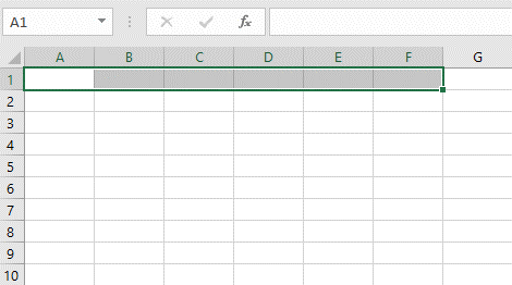
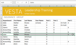
  1. Select the cell(s) with content you want to delete. In our example, we’ll select the cell range A10:H10.
  2. Select the Clear command on the Home tab, then click Clear Contents.

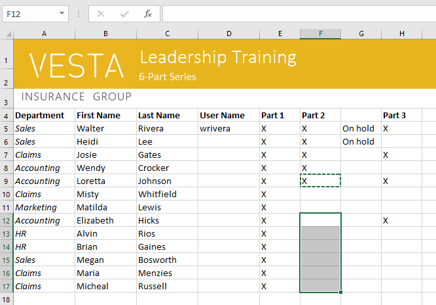
To copy and paste cell content:

Excel allows you to copy content that is already entered into your spreadsheet and paste that content to other cells, which can save you time and effort.

  1. Select the cell(s) you want to copy. In our example, we’ll select F9.
  2. Click the Copy command on the Home tab, or press Ctrl+C on your keyboard.
  3. Select the cell(s) where you want to paste the content. In our example, we’ll select F12:F17. The copied cell(s) will have a dashed box around them.

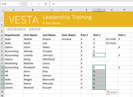
  4. Click the Paste command on the Home tab, or press Ctrl+V on your keyboard.

  5. The content will be pasted into the selected cells.

Working with Multiple Worksheets

When working with a large amount of data, you can create multiple worksheets to help organize your workbook and make it easier to find content. You can also group worksheets to quickly add information to multiple worksheets at the same time.

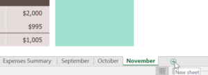
To insert a new worksheet:

Locate and select the New sheet button near the bottom-right corner of the Excel window.

new blank worksheet will appear.

To copy a worksheet:

If you need to duplicate the content of one worksheet to another, Excel allows you to copy an existing worksheet.

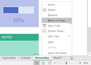
1. Right-click the worksheet you want to copy, then select Move or Copy from the worksheet menu.

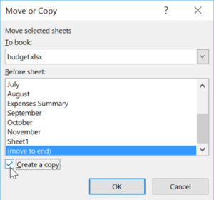
2. The Move or Copy dialog box will appear. Choose where the sheet will appear in the Before sheet: field. In our example, we’ll choose (move to end) to place the worksheet to the right of the existing worksheet.


3.  Check the box next to Create a copy, then click OK.

To rename a worksheet – select Rename from the worksheet menu.

1.3.1 Formulas

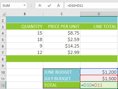
One of the most powerful features in Excel is the ability to calculate numerical information using formulas. Just like a calculator, Excel can add, subtract, multiply, and divide. In this lesson, we’ll show you how to use cell references to create simple

All formulas in Excel must begin with an equals sign (=). This is because the cell contains, or is equal to, the formula and the value it calculates.

Understanding cell references

While you can create simple formulas in Excel using numbers (for example, =2+2 or =5*5), most of the time you will use cell addresses to create a formula. This is known as making a cell reference. Using cell references will ensure that your formulas are always accurate because you can change the value of referenced cells without having to rewrite the formula.

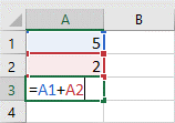
In the formula below, cell A3 adds the values of cells A1 and A2 by making cell references:

Type the equals sign (=). Notice how it appears in both the cell and the formula bar.

When you press Enter, the formula calculates and displays the answer in cell A3.

1.3.2 Functions

A function is a predefined formula that performs calculations using specific values in a particular order. Excel includes many common functions that can be used to quickly find the sum, average, count, maximum value, and minimum value for a range of cells. In order to use functions correctly, you’ll need to understand the different parts of a function and how to create arguments to calculate values and cell references.

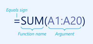
n order to work correctly, a function must be written a specific way, which is called the syntax. The basic syntax for a function is the equals sign (=), the function name (SUM, for example), and one or more arguments. Arguments contain the information you want to calculate. The function in the example below would add the values of the cell range A1:A20.

Working with arguments

Variety of functions available in Excel

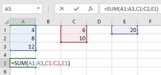
  • SUM: This function adds all of the values of the cells in the argument.
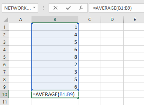
  • AVERAGE: This function determines the average of the values included in the argument. It calculates the sum of the cells and then divides that value by the number of cells in the argument.
  • COUNT: This function counts the number of cells with numerical data in the argument. This function is useful for quickly counting items in a cell range.
  • MAX: This function determines the highest cell value included in the argument.
  • MIN: This function determines the lowest cell value included in the argument.

AutoSum command

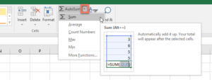
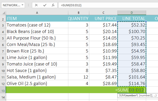
The AutoSum command allows you to automatically insert the most common functions into your formula, including SUM, AVERAGE, COUNT, MIN, and MAX. In the example below, we’ll use the SUM function to calculate the total cost for a list of recently ordered items.


Working with arguments

1. Select the cell that will contain the function. 

2. In the Editing group on the Home tab, click the arrow next to the AutoSum command. Next, choose the desired function from the drop-down menu. In our example, we’ll select Sum.2. 

3. Excel will place the function in the cell and automatically select a cell range for the argument.

Additionally, you can select the desired function from the drop-down menu:

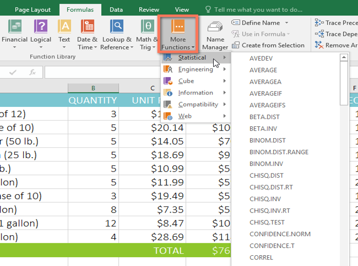
1. Click the Formulas tab on the Ribbon to access the Function Library.

2. From the Function Library group, select the desired function category. In the example,  More Functions are chosen, then hovered the mouse over Statistical.

1.5 Working with Data

Excel workbooks are designed to store a lot of information. Whether you’re working with 20 cells or 20,000, Excel has several features to help you organize your data and find what you need.

Freezing rows and columns

You may want to see certain rows or columns all the time in your worksheet, especially header cells. By freezing rows or columns in place, you’ll be able to scroll through your content while continuing to view the frozen cells. 

In the example below are frozen the top two rows, which allows you to view the dates no matter where you scroll in the spreadsheet.

To freeze rows:

  1. Select the row below the row(s) you want to freeze. In our example, we want to freeze rows 1 and 2, so we’ll select row 3.
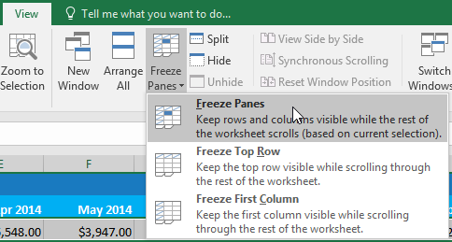
  2. On the View tab, select the Freeze Panes command, then choose Freeze Panes from the drop-down menu.
  3. The rows will be frozen in place, as indicated by the gray line. You can scroll down the worksheet while continuing to view the frozen rows at the top.

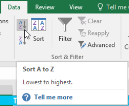
Sorting data

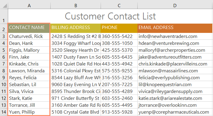
You can quickly reorganize a worksheet by sorting your data.  Content can be sorted alphabetically, numerically, and in many other ways. For example, you could organize a list of contact information by last name.

The worksheet will be sorted by the selected column. In our example, the worksheet is now sorted by Contact Name.


Filtering data

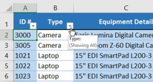
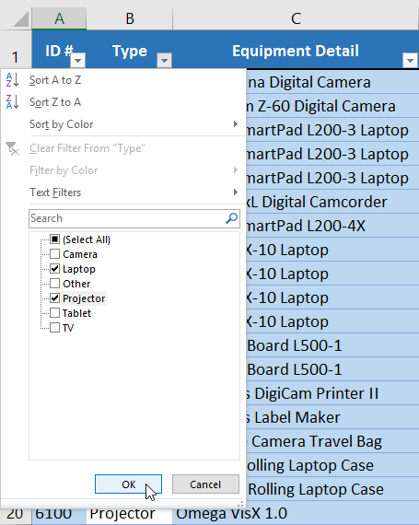
Filters can be used to narrow down the data in your worksheet, allowing you to view only the information you need. In this example, we’re filtering the worksheet to show only rows that contain the words Laptop or Projector in column B.

  1. In order for filtering to work correctly, your worksheet should include a header row, which is used to identify the name of each column.
  2. Select the Data tab, then click the Filter command.
  3. Click the drop-down arrow for the column you want to filter. In our example, we will filter column B to view only certain types of equipment.

Summarizing data

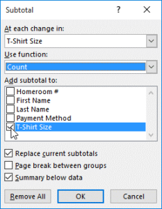
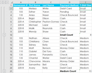
Excel allows you to quickly summarize your data. In the example below, created a subtotal for each T-shirt size, which makes it easy to see how many you‘ll need in each size.

  1. Sort your worksheet by the data you want to subtotal.
  2. Select the Data tab, then click the Subtotal command.
  3. The Subtotal dialog box will appear. Click the drop-down arrow for the At each change in: field to select the column you want to subtotal. In the example beside T-Shirt Size is selected.
  4. In the Add subtotal to: field, select the column where you want the calculated subtotal to appear. In our example, we’ll select T-Shirt Size. When you’re satisfied with your selections, click OK.

Formatting data as a table

ust like regular formatting, tables can improve the look and feel of your workbook, but they’ll also help you organize your content and make your data easier to use. For example, tables have built-in sorting and filtering options. Excel also includes several predefined table styles, allowing you to create tables quickly.

1. Select the cells you want to format as a table.   

2. From the Home tab, click the Format as Table command

3. Select a table style from the drop-down menu.

The cell range will be formatted in the selected table style.

Visualizing data with charts

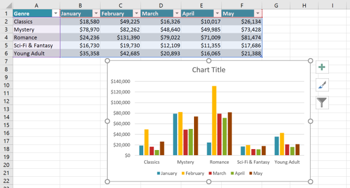
Charts allow you to illustrate your workbook data graphically, which makes it easy to visualize comparisons and trends.


To insert a chart:

  1. Select the cells you want to chart, including the column titles and row labels. These cells will be the source data for the chart. In the example, cells A1:F6 selected. 
  2. From the Insert tab, click the desired Chart command. In the example, select is Column.

*  If you’re not sure which type of chart to use, the Recommended Charts command will suggest several different charts based on the source data.

1.6 Using templates

template is a predesigned spreadsheet you can use to create a new workbook quickly. Templates often include custom formatting and predefined formulas, so they can save you a lot of time and effort when starting a new project.

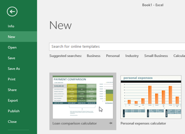
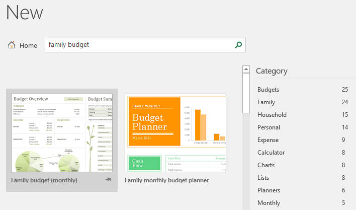
Click the File. Select New. Several templates will appear below the Blank workbook option.

Select a template to review it.

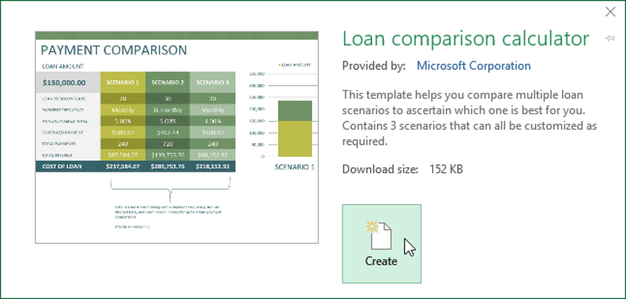
A preview of the template will appear, along with additional information on how the template can be used.

Click Create to use the selected template.

A new workbook will appear with the selected template.

You can also browse templates by category or use the search bar to find something more specific.

*  Select New and tap Home in the search field 

You can easily present and make calculations on Budget, Expenses, make Planners, Diagrams and etc. 

Note: not all templates are created by Microsoft. Many are created by third-party providers and even individual users, so some templates may work better than others.

1.7 Understanding OneDrive

Many of the features in Office are geared toward saving and sharing files online. 

OneDrive is Microsoft’s online storage space you can use to save, edit, and share your documents and other files.  You can access OneDrive from your computer, smartphone, or any of the devices you use.

To get started with OneDrive, all you need to do is set up a free Microsoft account. 

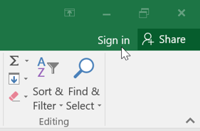
Once you have a Microsoft account, you’ll be able to sign in to Office. Just click Sign in in the upper-right corner of the Excel window.

Benefits of using OneDrive

Once you’re signed in to your Microsoft account, here are a few of the things you’ll be able to do with OneDrive:

Access your files anywhere: When you save your files to OneDrive, you’ll be able to access them from any computer, tablet, or smartphone that has an Internet connection. You’ll also be able to create new documents from OneDrive.

Back up your files: Saving files to OneDrive gives them an extra layer of protection. Even if something happens to your computer, OneDrive will keep your files safe and accessible.

Share files: It’s easy to share your OneDrive files with friends and coworkers. You can choose whether they can edit or simply read files. This option is great for collaboration because multiple people can edit a document at the same time (this is also known as co-authoring).

Saving and opening files

When you’re signed in to your Microsoft account, OneDrive will appear as an option whenever you save or open a file. You still have the option of saving files to your computer. However, saving files to your OneDrive allows you to access them from any other computer, and it also allows you to share files with friends and coworkers.

For example, when you click Save As, you can select either OneDrive or This PC as the save location.

To open an existing workbook:

In addition to creating new workbooks, you’ll often need to open a workbook that was previously saved.

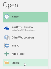
*  Navigate to Backstage view, then click Open.

*  Select Computer, then click Browse. Alternatively, you can choose OneDrive to open files stored on your OneDrive.

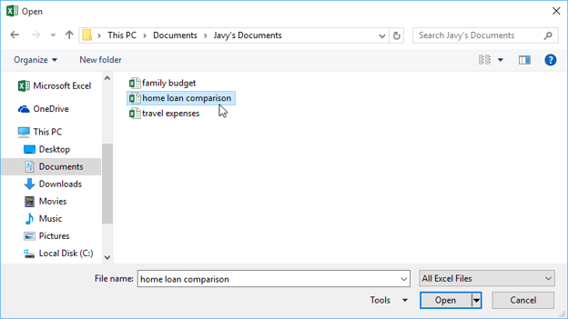
The Open dialog box will appear. Locate and select your workbook, then click Open.

*  If you’ve opened the desired workbook recently, you can browse your Recent Workbooks rather than search for the file.
 

SYNOPSIS

Excel is needed to work with data: make calculations, plans, illustrations; to schedule, manage and store information.

In an “Age of Information” ability to work with Excel enables smooth presentation and sharing of various data and information with your clients. 

The Beginner MS Excel training unit covers the various tools and formula you should know in your daily Excel work. The focus of the Beginner course is more on understanding the basics and essentials of MS Excel use.
Excel 2016″. GCF Global:Creating opportunities for a better life. Available at: https://edu.gcfglobal.org/en/excel2016/
Beginning Excel, First Edition”. Open Oregon. Available at:
https://openoregon.pressbooks.pub/beginningexcel/chapter/1-1-overview-of-microsoft-excel/

https://edu.gcfglobal.org/en/excel2016/getting-started-with-excel/1/